Note

Download full notebook here

Multi-Component Reflectance Model

This tutorial extends our single-species model to simulate reflectance from a planetary regolith that contains a mixture of materials. We will model a surface composed of H₂O and CO₂ ices, two species with distinct optical behaviors.

We will:

• Load optical constants for both H₂O and CO₂

• Configure their relative abundances and grain sizes

• Explore different mixing geometries (intimate vs. linear)

• Generate and visualize the resulting reflectance spectrum

This example helps illustrate how multiple species combine to shape the overall spectral response — and sets the stage for performing retrievals on more realistic data.

from importlib import reload
import numpy as np
import matplotlib.pyplot as plt
import matplotlib as mpl
import frostie.hapke as hapke
import frostie.utils as utils
mpl.rcParams['figure.dpi'] = 200
import os
import copy

As in the previous example, we will initialize a regolith object

example_two_regolith = hapke.regolith()

Next, we will load the optical constants of the two components

wav_water, n_water, k_water = utils.load_water_op_cons()
wav_co2, n_co2, k_co2 = utils.load_co2_op_cons()

Let’s plot these optical constants to get an intuition of how their absorption strength compares to each other

fig, ax = plt.subplots(nrows=1, ncols=2, figsize=(8,4))
ax[0].plot(wav_water,k_water, label='H$_2$O')
ax[0].plot(wav_co2,k_co2, label='CO$_2$')
ax[0].set_ylabel('k')
ax[0].set_yscale('log')
ax[0].set_xlabel('wavelength in $\mu$m')

ax[1].plot(wav_water,n_water, label='H$_2$O')
ax[1].plot(wav_co2,n_co2, label='CO$_2$')
ax[1].set_ylabel('n')
ax[1].set_xlabel('wavelength in $\mu$m')

# common legend for all subplots

handles, labels = ax[0].get_legend_handles_labels()
fig.legend(handles, labels, loc='upper center', ncol=3, bbox_to_anchor=(0.515, 1.1), fontsize=13)
plt.tight_layout();

Although CO₂ has several absorption features, its \(k\) values are generally much weaker than those of H₂O across most of the near-infrared. This means CO₂ contributes localized features while H₂O dominates the continuum.

Let’s now add these two components to our example_two_regolith object. Since there are multiple components in this regolith, we will need to also provide their abundance fractions as input. We will fix D and p_type

f = 0.5    # equal abundance (by number) fraction

water = {'name':'water','n':n_water, 'k':k_water, 'wav':wav_water, 'D':100, 'p_type':'HG2', 'f':f}
co2 = {'name':'carbon dioxide', 'n':n_co2, 'k':k_co2, 'wav':wav_co2, 'D':100, 'p_type':'HG2', 'f':f}

example_two_regolith.add_components([water, co2], matched_axes=False)

The matched_axes flag indicates whether all components share a common wavelength grid. If not, interpolation will be performed internally. While this step is optional for forward modeling, it becomes important for efficient model fitting.

Next, we set up the observation geometry, porosity, backscattering and internal-scattering parameters.

example_two_regolith.set_obs_geometry(i=45,e=45,g=90)

example_two_regolith.set_porosity(p=0.9)

example_two_regolith.set_backscattering(B=0)

example_two_regolith.set_s(s=0)

Finally, we need to decide the mixing mode of our components, i.e., whether they are mixed in an intimate way (also called salt-and-pepper model) or in a linear way (also called ‘areal’ model), as illustrated in the cartoon below:

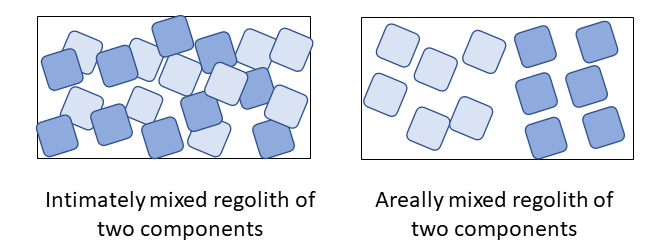
Let’s choose intimate mixing for now, as modeling the non-linear effects of mixing is one of the strengths of Hapke theory.

example_two_regolith.set_mixing_mode('intimate')

We are ready to model the reflectance spectrum of example_two_regolith!

example_two_regolith.calculate_reflectance()

plt.figure()
plt.plot(example_two_regolith.wav_model, example_two_regolith.model)
plt.ylabel('reflectance')
plt.xlabel('wavelength in $\mu$m')

This reflectance spectrum of a water and carbon dioxide mixture is pretty similar to the water ice reflectance spectrum from the previous example, except for sharp absorption features caused by carbon dioxide. This makes sense as water’s \(k\) spectrum is much stronger compared to carbon dioxide’s, so it is expected to dominate the continuum of the mixture spectrum.

Let’s also see how the linear mixing model differs from the intimate mixing model above

intimate_mix_regolith = copy.deepcopy(example_two_regolith)
linear_mix_regolith = copy.deepcopy(example_two_regolith)

linear_mix_regolith.set_mixing_mode('linear')
linear_mix_regolith.calculate_reflectance()

plt.figure()
plt.plot(intimate_mix_regolith.wav_model, intimate_mix_regolith.model, label='intimate')
plt.plot(linear_mix_regolith.wav_model, linear_mix_regolith.model, label='linear')
plt.ylabel('reflectance')
plt.xlabel('wavelength in $\mu$m')
plt.legend()

<matplotlib.legend.Legend at 0x1225c7390>

Summary

In this tutorial, we extended our Hapke-based reflectance modeling to simulate a regolith containing multiple components — specifically, a mixture of H₂O and CO₂ ices. We explored how the individual optical constants of each species contribute to the overall reflectance spectrum, and how their relative abundances, grain sizes, and mixing geometry shape the resulting spectral features.

Key takeaways:

• The Hapke model can simulate both intimate and linear mixing modes, capturing non-linear effects that arise when particles are physically mixed.

• Dominant species (like H₂O in this case) control the continuum shape, while weaker components (like CO₂) introduce localized absorptions.

• Matching the wavelength axes of all components ensures accurate and efficient spectrum computation.

In the next tutorial, we will explore how to go beyond forward modeling and use Bayesian inference to retrieve the composition and physical properties of a surface directly from observed spectra.